Early Warning Signals for Critical Transitions
PhD Thesis — University of Reading, Department of Mathematics and Statistics. Published in EPL (Europhysics Letters), Chaos, and Environmental Research Letters. Read the thesis.
The Big Picture
Many complex systems in nature — from ecosystems to climate to financial markets — can undergo sudden, dramatic shifts known as tipping points or critical transitions. A lake can flip from clear to turbid seemingly overnight. The Sahara transformed from a green savanna to desert over just a few centuries. The 2008 financial crisis cascaded through the global economy in weeks.
The question that drove my PhD research was: Can we detect warning signs before these catastrophic shifts occur? It turns out that many systems exhibit characteristic behaviours as they approach a tipping point — a phenomenon called critical slowing down.

Critical Slowing Down
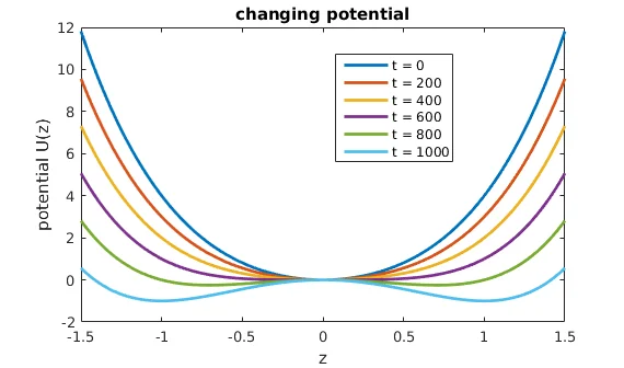
Imagine a ball sitting in a bowl. Push it slightly and it rolls back to the centre. Now imagine the bowl slowly becoming flatter. The ball still returns to equilibrium, but more slowly. Eventually, when the bowl is nearly flat, even a small push sends the ball over the edge.
This is critical slowing down: as a system approaches a tipping point, it takes longer to recover from perturbations. This manifests in measurable statistical properties of the system's time series:
- Increased autocorrelation — the system's state becomes more similar to its recent past
- Increased variance — fluctuations grow larger as stability weakens
- Spectral reddening — low-frequency variations dominate the signal
Early Warning Signal Indicators
My research focused on developing and comparing methods to detect critical slowing down in time series data. The core technique is sliding window analysis: calculate a statistical indicator in overlapping windows of data to track how it changes over time. A rising trend in the indicator can serve as an early warning signal.
ACF1 Indicator (Lag-1 Autocorrelation)
The most established indicator measures how correlated a time series is with itself at a one-step lag. As critical slowing down increases, the system "remembers" its past state longer, and autocorrelation rises toward 1.
DFA Indicator (Detrended Fluctuation Analysis)
DFA quantifies long-range correlations by measuring how fluctuations scale with time window size. It's particularly useful for non-stationary signals where simple autocorrelation may be misleading. This method was developed for tipping point analysis by Livina and colleagues.
PS Indicator (Power Spectrum Scaling)
A novel contribution of my thesis was using the power spectrum scaling exponent as an early warning indicator. By transforming the time series to the frequency domain and measuring how power scales with frequency, we can detect the "reddening" of the spectrum that accompanies critical slowing down.
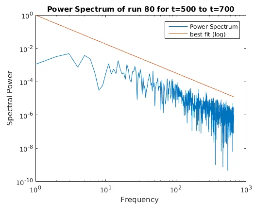
The key insight is that all three indicators are mathematically related for autoregressive processes, but the PS indicator has a practical advantage: it's insensitive to periodic components in the data, making it useful for signals with daily or seasonal cycles.
Types of Tipping Points
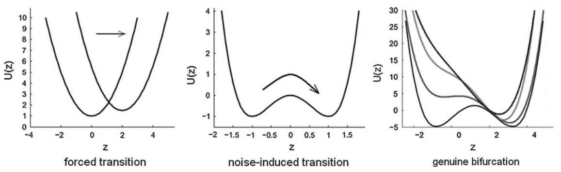
Not all tipping points are alike. My thesis examined three categories:
| Type | Mechanism | EWS Detectable? |
|---|---|---|
| Bifurcational | Stable state disappears as parameters change | Yes |
| Noise-induced | Random fluctuations push system to alternate state | Limited |
| Forced transition | External forcing shifts the equilibrium | Sometimes |
Multidimensional Systems
Real-world systems rarely have just one variable. Climate involves temperature, pressure, humidity, and countless other factors. My thesis extended the one-dimensional EWS techniques to handle multivariate data using two approaches:
Empirical Orthogonal Functions (EOFs)
EOF analysis (equivalent to Principal Component Analysis) finds the linear combination of variables that captures the most variance. An important theoretical contribution of my thesis was proving that the EOF projection is optimal not just for capturing variance, but specifically for detectingincreases in variance — exactly what we need for early warning signals.
Jacobian Eigenvalue Analysis
For systems where we can estimate the dynamics, tracking the eigenvalues of the Jacobian matrix directly reveals approaching bifurcations. When an eigenvalue crosses from negative to positive real part, the system becomes unstable.
Application: Tropical Cyclones
To test these methods on real geophysical data, I applied them to an unconventional problem: detecting the approach of tropical cyclones from sea-level pressure measurements. While not a classical bifurcation, the sudden drop in pressure as a hurricane arrives is certainly an "abrupt change" in the system.

I analysed 14 major tropical cyclones using data from HadISD weather stations, examining sea-level pressure time series in the days before landfall. Key findings:
- The PS indicator showed rising trends 24-48 hours before the pressure drop
- The ACF1 indicator was confounded by 12-hour tidal oscillations in the pressure data
- Spatial analysis of multiple weather stations revealed the approaching storm as a "wave" of increasing indicator values

I also developed a stochastic model of hurricane approach, parameterised using the observed EWS indicator behaviour. This model successfully reproduced the statistical signatures seen in real data, validating the use of these indicators for this application.
Climate Applications
Beyond tropical cyclones, my research connected to broader climate tipping point research. The same techniques can potentially detect warning signs for major climate transitions:
- Atlantic thermohaline circulation collapse — slowdown of the Gulf Stream
- Arctic sea ice loss — ice-albedo feedback instability
- Amazon rainforest dieback — precipitation-vegetation feedback
- Sahara greening/desertification — vegetation-climate coupling
Publications
Paper 1 — EPL (Europhysics Letters)
"A novel scaling indicator of early warning signals helps anticipate tropical cyclones"
Introduced the PS indicator and demonstrated its use on model systems and tropical cyclone data.
Paper 2 — Chaos
"Generalized early warning signals in multivariate and gridded data with an application to tropical cyclones"
Extended EWS methods to multivariate systems using EOF analysis and spatial gridded data.
Paper 3 — Environmental Research Letters
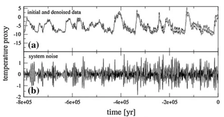
"Early warning signals of the termination of the African Humid Period"
Applied EWS techniques to paleoclimate data to study the desertification of the Sahara.
Codebase & Implementation
The analysis was primarily conducted in MATLAB with supplementary Python scripts. I developed a modular codebase with reusable functions for calculating EWS indicators, integrating stochastic differential equations, and analysing multivariate time series.
Repository Structure
MatlabCode/
├── Core_Functions/
│   ├── Indicator_methods/
│   │   ├── Scaling/          # ACF, DFA, PSE core algorithms
│   │   └── Sliding_window/   # Sliding window implementations
│   ├── Dynamical_Systems/    # Hopf, homoclinic, Van der Pol
│   ├── NumericalIntegration/ # Milstein SDE solver
│   └── Statistics/           # Mann-Kendall trend test
├── Projects/
│   ├── Paper2018_EPL/        # Scaling indicators paper
│   ├── Paper2019_Multidim/   # Multivariate EWS paper
│   └── Thesis/               # Thesis chapter code
├── Data/
│   ├── HadISD/               # Weather station data
│   └── Ice_Cycles/           # Paleoclimate records
└── Tests/                    # Unit tests
Core Indicator Functions
The three main EWS indicators are implemented as standalone functions that can be applied to any time series:
| Function | Description | EWS Threshold |
|---|---|---|
| ACF.m | Lag-k autocorrelation | ACF(1) → 1 |
| DFA.m | Detrended Fluctuation Analysis | α → 1.5 |
| PSE.m | Power Spectrum Exponent | β → 2 |
| VAR_sliding.m | Sliding window variance | σ² → ∞ |
ACF Implementation
The autocorrelation function measures how correlated a time series is with a lagged version of itself:
function auto_corr = ACF(data, lag)
%% ACF Compute autocorrelation at a given lag
%
% Formula: ACF(k) = E[(X_t - μ)(X_{t+k} - μ)] / Var(X)

    m = mean(data);
    n = size(data, 1);

    data1 = data(1:n-lag) - m;
    data2 = data(1+lag:n) - m;

    auto_corr = mean(data1 .* data2) / var(data);
end
DFA Implementation
Detrended Fluctuation Analysis quantifies long-range correlations by measuring how the RMS fluctuation scales with segment length. The algorithm divides the cumulative sum (profile) into segments, fits a polynomial trend to each, and computes the residual variance:
function F = DFA(data, segment_len, order)
%% DFA - Measures long-range correlations
% Reference: Peng et al. (1994)

% Step 1: Compute cumulative sum (profile)
N = size(data, 1);
Y = cumsum(data);

% Step 2: Divide into segments and detrend
Ns = floor(N / segment_len);
Fs = zeros(Ns, 1);

for nu = 1:Ns
    indices = ((nu-1)*segment_len + 1 : nu*segment_len)';

    % Fit polynomial and compute residuals
    poly = polyfit(indices, Y(indices), order);
    trend = polyval(poly, indices);
    residuals = Y(indices) - trend;

    % Segment variance
    Fs(nu) = mean(residuals.^2);
end

% Step 3: RMS fluctuation
F = sqrt(mean(Fs));
end
The DFA exponent α is estimated by computing F(s) for multiple segment lengths and fitting log(F) vs log(s). For white noise α ≈ 0.5; for random walk α ≈ 1.5.
PSE Implementation (Novel Contribution)
The Power Spectrum Exponent estimates β from the slope of the power spectrum in log-log space. A key insight was selecting the appropriate frequency range for fitting:
function pse_value = PSE(Y)
%% PSE - Estimate β from power spectrum slope
% For S(f) ~ f^(-β): β=0 for white noise, β=2 for Brownian motion

    % Compute periodogram
    [pxx, f] = periodogram(Y, [], [], 1);

    % Remove DC component
    f = f(2:end);
    pxx = pxx(2:end);

    % Fit line in log-log space
    % Frequency range [0.01, 0.1] chosen for AR(1) processes
    window = (f <= 0.1) & (f >= 0.01);

    logf = log10(f(window));
    logp = log10(pxx(window));

    pfit = polyfit(logf, logp, 1);
    pse_value = -pfit(1);  % Negative slope = positive β
end
Sliding Window Analysis
To track indicator evolution over time, each function has a sliding window variant:
function slidingACF = ACF_sliding(data, lag, windowSize)
%% Compute ACF in sliding windows across the time series

    n = size(data, 1);
    slidingACF = zeros(n, 1);

    for i = (windowSize + 1):n
        window = data((i - windowSize):i);
        slidingACF(i) = ACF(window, lag);
    end
end
Numerical Integration of SDEs
Test systems were integrated using the Milstein method for stochastic differential equations of the form dX = f(X,t)dt + σdW. The implementation handles both constant and time-varying noise amplitudes:
function [t, Y] = milstein(f, sigma, x0, tBounds, dt)
%% Milstein method for SDEs: dX = f(X,t)dt + σdW

N = floor((tBounds(2) - tBounds(1)) / dt);
t = linspace(tBounds(1), tBounds(2), N)';
m = size(x0, 1);   % System dimension
Y = zeros(m, N);
Y(:,1) = x0;

for i = 2:N
    dW = randn(m, 1);  % Brownian increment

    % Euler-Maruyama step
    Y(:,i) = Y(:,i-1) + f(Y(:,i-1), t(i-1))*dt ...
             + sqrt(dt) * sigma * dW;
end
end
Test Systems
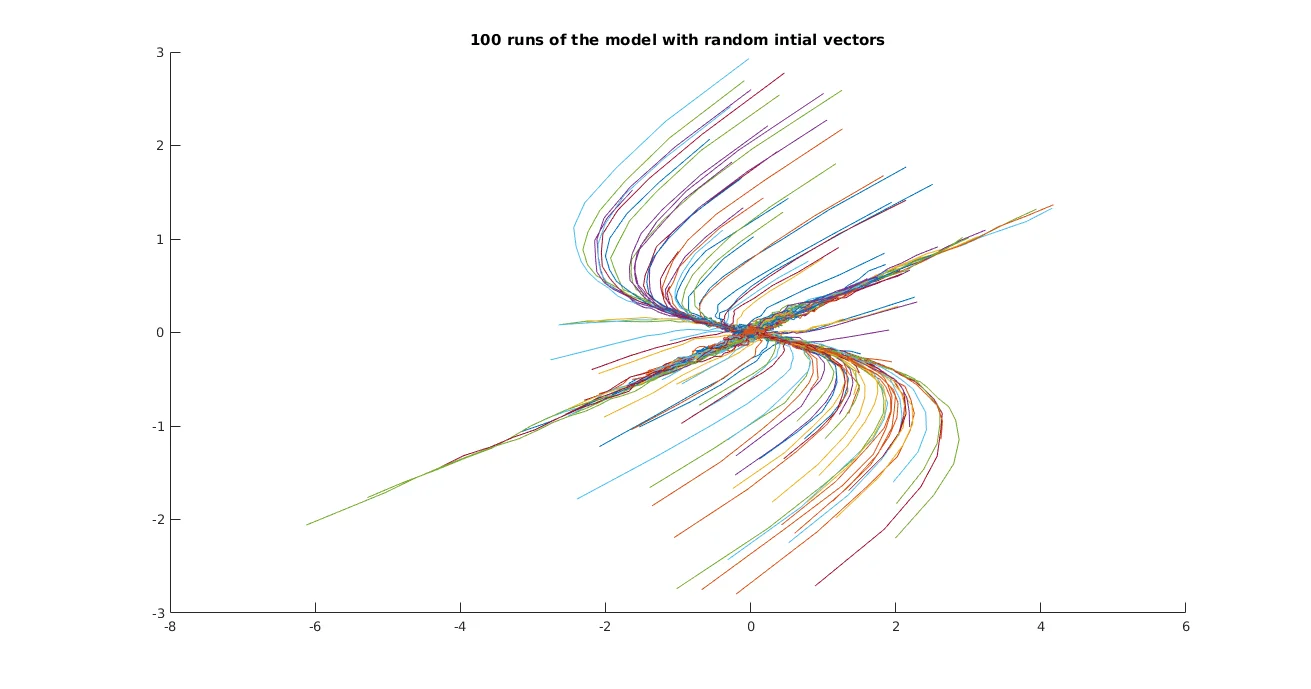
I implemented several dynamical systems to validate EWS methods under controlled conditions:
% Hopf bifurcation: stable equilibrium → limit cycle
% System: dr/dt = μr - r³,  dθ/dt = ω

x0 = [0.001; 0];  % Start near origin
T_end = 65;

% μ increases from -2.9 to 0.2 (crosses bifurcation at μ=0)
mu = @(t) -2.9 + 0.05*t;

[t, r] = hopf_fun(0, T_end, x0, mu, 0.01);

% Convert to Cartesian for analysis
x = r(:,1) .* cos(r(:,2));
y = r(:,1) .* sin(r(:,2));

% Apply EWS indicators
acf1 = ACF_sliding([x, y], 1, 100);
dfa_alpha = DFA_sliding([x, y], 2, 100);
The AR(1) Model for Critical Slowing Down
Critical slowing down is often modelled as a first-order autoregressive process:
where η(t) is Gaussian white noise. As μ approaches 1, the process becomes more "memory-like" — perturbations persist longer before decaying. The power spectrum of this process is:
A key theoretical contribution was showing that even though this doesn't exhibit true power-law scaling, fitting a scaling exponent β still provides a monotonically increasing indicator as μ → 1, making it valid for EWS detection.
EOF Analysis for Multivariate Data
function eof_ts = EOF_sliding(data, windowSize)
%% Project multivariate data onto principal component

    [n, dim] = size(data);
    eof_ts = zeros(n, 1);

    for i = (windowSize + 1):n
        window = data((i - windowSize):i, :);

        % Compute covariance matrix
        C = cov(window);

        % Find eigenvector with largest eigenvalue
        [V, D] = eig(C);
        [~, idx] = max(diag(D));

        % Project current point onto EOF
        eof_ts(i) = data(i, :) * V(:, idx);
    end
end
Usage Example
%% Generate test data with increasing autocorrelation
N = 1000;
phi = linspace(0.5, 0.95, N);  % AR(1) coefficient → 1
data = zeros(N, 1);

for i = 2:N
    data(i) = phi(i) * data(i-1) + randn;
end

%% Calculate sliding window indicators
windowSize = 100;

acf1 = ACF_sliding(data, 1, windowSize);
dfa_alpha = DFA_sliding(data, 2, windowSize);
pse_beta = PSE_sliding(data, windowSize);
variance = VAR_sliding(data, windowSize);

%% Statistical significance: Mann-Kendall trend test
[~, p_acf] = mannkendall(acf1(windowSize+1:end));
[~, p_dfa] = mannkendall(dfa_alpha(windowSize+1:end));
[~, p_pse] = mannkendall(pse_beta(windowSize+1:end));

%% Plot results
figure
subplot(4,1,1); plot(data); ylabel('Data')
subplot(4,1,2); plot(acf1); ylabel('ACF(1)')
subplot(4,1,3); plot(dfa_alpha); ylabel('DFA α')
subplot(4,1,4); plot(pse_beta); ylabel('PSE β')
Key Contributions
- Developed the Power Spectrum (PS) scaling indicator as a novel EWS method
- Proved theoretical validity of PS indicator for non-power-law-scaling processes
- Justified EOF dimension reduction for variance-based EWS detection
- Applied EWS methods to tropical cyclone prediction — a novel application domain
- Developed a stochastic hurricane model parameterised by EWS indicators
- Published three peer-reviewed papers in physics and climate journals
Reflections
This PhD taught me that the most interesting problems often lie at the boundaries between fields. Tipping point theory draws on dynamical systems, statistics, time series analysis, and domain-specific knowledge from climate science to ecology. The mathematical beauty of critical slowing down is that the same signatures appear in systems as different as lakes, climate, and financial markets.
The practical challenge is that real data is messy. Periodicities, non-stationarity, measurement noise, and finite sample sizes all conspire against clean detection. My work on the PS indicator was partly motivated by the real-world problem of 12-hour tidal oscillations corrupting the autocorrelation signal in sea-level pressure data.
Perhaps the most important lesson: early warning signals are not predictions. They indicate increased risk, not certainty. A rising indicator means "the system is losing resilience" — whether or not a tipping point actually occurs depends on factors we may not be measuring.