Fraud Detection
The Problem
The IEEE-CIS Fraud Detection Kaggle competition from 2019 caught my eye as an interesting side project. What drew me in was the combination of challenges that make fraud detection genuinely tricky: severe class imbalance (only 3.5% of transactions are fraudulent), high dimensionality (590K transactions with 450+ features), and hundreds of anonymized features whose meaning must be inferred from patterns in the data.
Beyond the technical challenges, fraud detection presents an interesting business problem: aggressive prevention blocks legitimate customers, while lenient policies increase losses. You have to find the right trade-off. I was curious to see how far I could push a fairly simple approach, and the results turned out better than I expected: 97.4% AUC on holdout data and, with some reasonable cost assumptions, potential savings of around $447K compared to no model at all.
Exploratory Data Analysis
The dataset comes from Vesta Corporation and contains real e-commerce transactions. There are two tables: transaction data (590K rows, 394 columns) and identity data (144K rows, 41 columns). The identity data only exists for about 24% of transactions. Interestingly, transactions with identity data have a higher fraud rate (7.8%) than those without (2.1%). Counterintuitive, but it probably reflects that identity verification is triggered when fraud detection systems flag something suspicious.
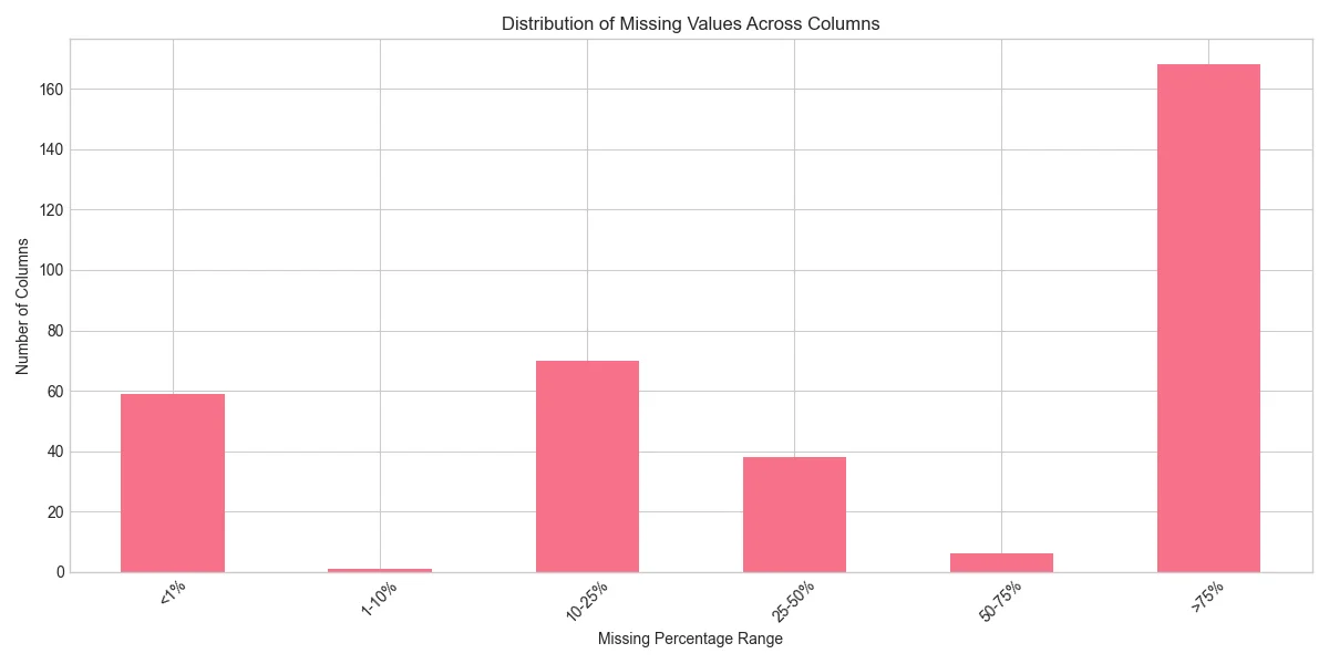
A significant portion of the features are anonymized: 339 "V" features (Vesta's proprietary engineered features), 14 "C" features (counts), and 15 "D" features (time deltas). With no documentation on what these mean, the only option is to analyse their distributions and correlations with fraud to infer their usefulness. Missing values are pervasive: 374 of 395 columns have at least some nulls, with many exceeding 50%:
Temporal Patterns
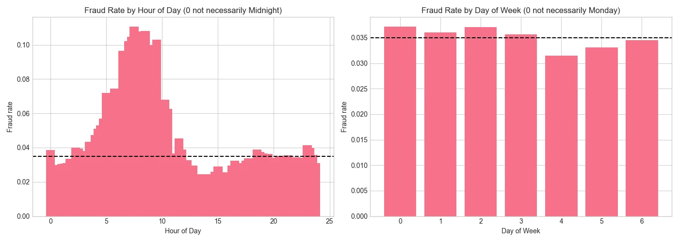
Fraud rates vary significantly by time of day. The plot below shows fraud rate binned by hour—there's a clear cyclical pattern, though without knowing the actual timezone we can't say whether fraud peaks at night or during business hours. What matters is that the pattern exists and can be captured:
Email Domain Signals
One of the most striking findings was the email domain matching pattern. When the purchaser's email domain (P_emaildomain) matches the recipient's (R_emaildomain), the fraud rate jumps to 9.7%, compared to just 2.2% when they differ. This makes sense: legitimate purchases often involve shipping to someone else (gifts, different delivery address), while fraudsters typically ship to themselves.
# From EDA notebook
train['email_match'] = train['P_emaildomain'] == train['R_emaildomain']
fraud_by_email = train.groupby('email_match')['isFraud'].mean()

# Results:
# email_match
# False    0.022070   (2.2% fraud rate)
# True     0.096504   (9.7% fraud rate - 4.4x higher!)
Similarly, new cards showed elevated fraud rates. The D1 feature represents "days since card was first used", and cards less than 7 days old had notably higher fraud rates than established cards. Mobile devices also showed 10.2% fraud versus 6.5% for desktop (about 1.6x higher).
Identity Features: Not What They Seem
The identity table contains 38 id_XX columns, many with numeric dtypes. But plotting their distributions reveals that most aren't truly continuous—they have discrete peaks suggesting categorical meaning:

Take id_32: it only has 4 unique values (0, 16, 24, 32), probably screen color depth. Treating this as continuous would be misleading; it should be label-encoded. Similarly, columns like id_01, id_05, and id_06 show discrete peaks rather than smooth distributions, so frequency encoding works better. Only a handful (id_02, id_07, id_08) show genuinely continuous distributions and can be left as-is.
V Feature Block Structure
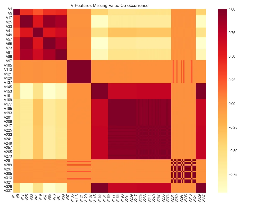
For the 339 anonymized V features, I analysed their missing value patterns. The heatmap revealed clear block structure: features V1-V11 are always missing together, V12-V34 form another block, and so on. This suggests Vesta collected these features in groups, and knowing which block is missing could be more predictive than just counting missing values.
Feature Engineering
Based on the EDA insights, I built a feature engineering pipeline using scikit-learn transformers. This keeps the code modular and ensures the same transformations are applied consistently to training and test data.
Cyclical Time Encoding
The transaction timestamp is given as seconds from some reference point. To capture daily and weekly patterns without the model thinking hour 23 and hour 0 are far apart, I used sine/cosine encoding:
class TimeFeatures(BaseEstimator, TransformerMixin):
    """Add cyclical time features from TransactionDT."""

    def transform(self, X):
        X = X.copy()
        hour = (X['TransactionDT'] / 3600) % 24
        day = (X['TransactionDT'] / 86400) % 7

        # Sine/cosine encoding preserves cyclical relationships
        # Hour 23 and hour 0 are now neighbors (both map to similar values)
        X['hod_sin'] = np.sin(2 * np.pi * hour / 24)
        X['hod_cos'] = np.cos(2 * np.pi * hour / 24)
        X['dow_sin'] = np.sin(2 * np.pi * day / 7)
        X['dow_cos'] = np.cos(2 * np.pi * day / 7)

        return X
Customer-Level Aggregations
The dataset doesn't have an explicit customer ID, but we can construct one from card and address information. With this pseudo-UID, we can compute each customer's typical spending pattern and flag transactions that deviate from it:
class AggregationFeatures(BaseEstimator, TransformerMixin):
    """Statistics per customer UID to detect unusual spending."""

    def __init__(self, uid_cols=None):
        self.uid_cols = uid_cols or ['card1', 'addr1']

    def fit(self, X, y=None):
        X = X.copy()
        X['_uid'] = self._create_uid(X)

        # Calculate per-customer statistics from training data
        self.uid_stats_ = X.groupby('_uid')['TransactionAmt'].agg(
            ['mean', 'std', 'count']
        )
        return self

    def transform(self, X):
        X = X.copy()
        X['_uid'] = self._create_uid(X)

        # Merge customer statistics
        X = X.merge(self.uid_stats_, left_on='_uid', right_index=True, how='left')

        # Z-score: how unusual is this transaction for this customer?
        X['amt_zscore'] = (
            (X['TransactionAmt'] - X['amt_mean']) /
            X['amt_std'].clip(lower=1e-6)
        )
        return X
This is based on insights from top Kaggle solutions. The 1st place solution used['card1', 'addr1', 'P_emaildomain'] as their customer identifier—I kept it simpler with just card and address.
Amount Patterns
EDA revealed a non-monotonic relationship between transaction amount and fraud rate: it increases from 2.4% ($0-25) to 5.5% ($500-1000), but then drops back to 3.4% for $1000+. Explicit amount buckets help tree models find these patterns. I also added cents-based features—fraudsters often use round amounts or specific patterns like $X.99:
class AmountFeatures(BaseEstimator, TransformerMixin):
    AMT_BINS = [0, 25, 50, 100, 200, 500, 1000, float('inf')]

    def transform(self, X):
        X = X.copy()

        X['TransactionAmt_log'] = np.log1p(X['TransactionAmt'])
        X['amt_bucket'] = np.digitize(X['TransactionAmt'], bins=self.AMT_BINS) - 1

        # Cents analysis (fraud detection best practice)
        cents = (X['TransactionAmt'] * 100 % 100).astype(int)
        X['cents'] = cents
        X['cents_00'] = (cents == 0).astype(int)  # Round amounts
        X['cents_99'] = (cents == 99).astype(int)  # Fake pricing pattern

        return X
Two Encoding Pipelines
I built two separate pipelines: one using label encoding for tree-based models (LightGBM can learn arbitrary splits on numeric values), and one using one-hot encoding for linear models (which would incorrectly interpret label-encoded categories as ordinal). The tree pipeline produced 484 features; the linear pipeline expanded to 613 due to one-hot encoding.
Modeling Approach
Why Time-Based Cross-Validation?
Standard k-fold cross-validation randomly shuffles data, letting the model "peek" at future fraud patterns when training. This inflates performance estimates unrealistically. In production, we can only use historical data to predict future transactions.
TimeSeriesSplit trains on earlier transactions and validates on later ones, which mirrors production deployment. It also helps detect concept drift: fraudsters constantly adapt their tactics, so a model trained on January data might perform differently on March data.
from sklearn.model_selection import TimeSeriesSplit

# Data is already sorted by TransactionDT
tscv = TimeSeriesSplit(n_splits=5)

for fold, (train_idx, val_idx) in enumerate(tscv.split(X_train)):
    # Each fold trains on EARLIER data, validates on LATER data
    # Fold 1: Train on 0-100k,  validate on 100k-200k
    # Fold 2: Train on 0-200k,  validate on 200k-300k
    # ...and so on
Model Comparison
I compared Logistic Regression (baseline) against LightGBM. LightGBM was a natural choice for this problem: it handles missing values natively (no imputation needed for 374 columns with nulls), works well with categorical features, and the scale_pos_weight parameter handles class imbalance.
params = {
    'objective': 'binary',
    'metric': 'auc',
    'boosting_type': 'gbdt',
    'scale_pos_weight': 27.58,  # (569877 legitimate) / (20663 fraud)
    'learning_rate': 0.05,
    'num_leaves': 31,
    'feature_fraction': 0.8,
    'bagging_fraction': 0.8,
    'bagging_freq': 5,
}
LightGBM significantly outperformed logistic regression: 0.9088 AUC vs 0.8423 (a 7.9% improvement). The gap was consistent across all five CV folds.

Cost-Benefit Optimization
This is where things get interesting. Traditional ML metrics like F1 score balance precision and recall equally, but the business costs aren't symmetric. I defined a simple cost matrix based on reasonable assumptions:
| Outcome | Cost | Rationale |
|---|---|---|
| False Negative (missed fraud) | $150 | Average fraud amount |
| False Positive (blocked legitimate) | $10 | Customer friction, lost goodwill |
| True Positive (caught fraud) | $5 | Manual review cost |
With these costs, I swept through different classification thresholds to find the one that minimizes total cost:
def calculate_cost(y_true, y_pred, costs):
    tn, fp, fn, tp = confusion_matrix(y_true, y_pred).ravel()
    total_cost = (
        fn * costs.false_negative_cost +  # $150 per missed fraud
        fp * costs.false_positive_cost +  # $10 per blocked legitimate
        tp * costs.true_positive_cost     # $5 per caught fraud
    )
    return total_cost

# Sweep thresholds
for thresh in np.arange(0.01, 0.99, 0.01):
    y_pred = (y_pred_proba >= thresh).astype(int)
    cost = calculate_cost(y_holdout, y_pred, costs)
    # Track minimum...
The results were revealing: the F1-optimal threshold was 0.82, but the cost-optimal threshold was 0.54. That's a huge difference! The lower threshold catches more fraud (higher recall) at the expense of more false positives—but given that a missed fraud costs 15x more than a blocked legitimate transaction, this is the right trade-off.
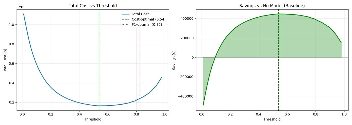
At the cost-optimal threshold, the model achieves 73% cost reduction compared to approving all transactions (the "no model" baseline). On this dataset, that translates to roughly $447K in savings, from $610K baseline cost down to $163K with the model.
Results
The final model achieves excellent class separation. The score distribution plot shows fraud transactions concentrated near 1.0 and legitimate transactions near 0.0, with relatively little overlap:
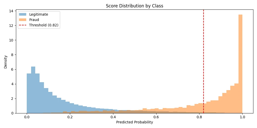
The ROC and Precision-Recall curves tell a similar story. The ROC-AUC of 0.9738 indicates excellent discrimination ability. The PR curve is particularly informative for imbalanced datasets: a PR-AUC of 0.7369 is strong given the 3.5% base rate (the baseline for a random classifier would be just 0.035).

Feature importance analysis confirmed that Vesta's anonymized features (V258, V294) are highly predictive, which isn't surprising given they've been engineered specifically for fraud detection. My engineered features also ranked highly: card1_addr1_amt_mean (customer average spend) and card1_freq (how common is this card) both appeared in the top 20.
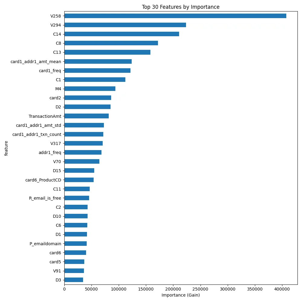
The top 93 features (of 484) account for 90% of total importance, which suggests plenty of room for model simplification in production. Fewer features means faster inference and easier maintenance.
Summary
- ROC-AUC (Holdout): 0.9738
- PR-AUC: 0.7369
- CV Mean AUC: 0.9088 ± 0.01
- F1-optimal threshold: 0.82 | Cost-optimal threshold: 0.54
- Cost Reduction: 73% vs. no model
- Estimated Savings: $446,985
Takeaways
The biggest lesson here was about framing the problem correctly. Optimizing for F1 score would have given a threshold of 0.82, missing 18% of fraud. Optimizing for business cost gave 0.54, catching significantly more fraud at an acceptable false positive rate.
In production you'd want to refine the cost assumptions with actual business data and monitor for concept drift (fraud patterns change!). But as a weekend project to explore cost-sensitive classification, I'm happy with how it turned out.