Multivariate Early Warning Signals
Published in Chaos (AIP Publishing), 2019. Read the paper.
Authors: J. Prettyman, T. Kuna, V. Livina
Summary
Real-world dynamical systems rarely involve just one variable. Climate involves temperature, pressure, humidity, and countless other factors. This paper extends early warning signal (EWS) techniques from one-dimensional time series to multivariate and spatially distributed data.
The key contributions are: (1) an analytical justification for using Empirical Orthogonal Functions (EOF) for dimension reduction in EWS contexts, (2) extension of EWS techniques to 2D spatial fields, and (3) development of astochastic model of a moving cyclone to validate these methods.
The Challenge of Multidimensional Data
Standard EWS indicators (variance, autocorrelation, scaling exponents) are designed for univariate time series. When we have multiple variables or spatially distributed measurements, we need strategies to either:
- Reduce dimensionality to apply 1D techniques to a derived signal
- Extend the indicators to work directly with multivariate data
- Analyse spatial patterns across multiple measurement locations
Empirical Orthogonal Functions (EOF)
The EOF method (also known as Principal Component Analysis) projects multidimensional data onto a new basis that maximises variance. The first EOF captures the direction of maximum variability in the system.
A natural question arises: Does the component with maximum variance also capture the early warning signal? After all, what matters for EWS detection is not variance itself, but the change in variance (or autocorrelation) as the system approaches a tipping point.
Theoretical Justification
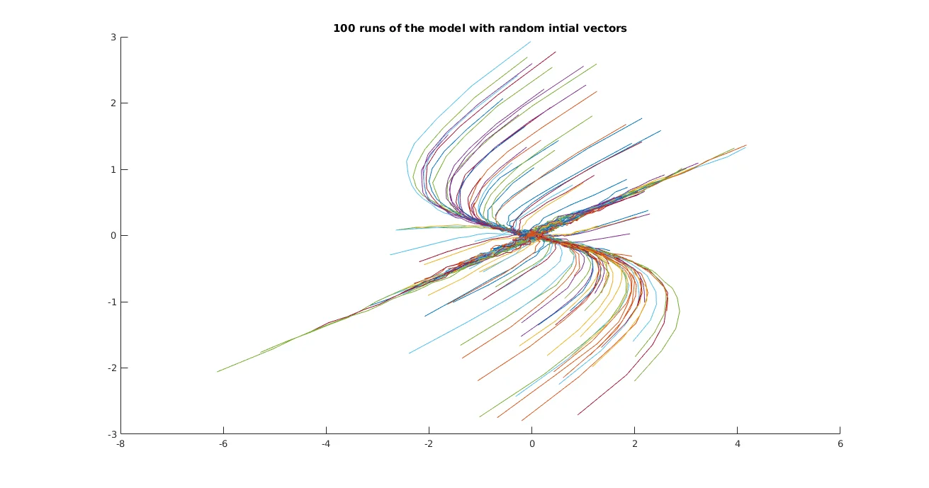
I proved analytically that for a general linear dynamical system approaching bifurcation, the first EOF loading vector tends to align with the eigenvector corresponding to the critical mode — exactly where the EWS will be observed.
Consider a discrete dynamical system:
where B is a contracting matrix with eigenvalue λ₁ approaching 1 (the bifurcation point). The covariance matrix of the system state is:
As λ₁ → 1, the term (1 - λ₁²)⁻¹ dominates, and the principal eigenvector of E[C] aligns with the first eigenvector of B — precisely the direction where the bifurcation will occur.
function eof_ts = EOF_sliding(data, windowSize)
%% Project multivariate data onto principal component

    [n, dim] = size(data);
    eof_ts = zeros(n, 1);

    for i = (windowSize + 1):n
        window = data((i - windowSize):i, :);

        % Compute covariance matrix
        C = cov(window);

        % Find eigenvector with largest eigenvalue
        [V, D] = eig(C);
        [~, idx] = max(diag(D));

        % Project current point onto EOF
        eof_ts(i) = data(i, :) * V(:, idx);
    end
end
The Williamson Method: Direct Jacobian Estimation
An alternative approach directly estimates the Jacobian eigenvalues from multivariate time series data. This method, introduced by Williamson et al., extends the 1D autocorrelation concept to multiple dimensions.
The matrix A is computed as a higher-dimensional analogue of the lag-1 autocorrelation:
The eigenvalues of A relate to the Jacobian eigenvalues via:
As the system approaches a bifurcation, the real part of the leading Jacobian eigenvalue crosses from negative to positive, providing a direct indicator of the approaching instability.
Application to Tropical Cyclone Data
Both methods were tested on sea-level pressure (SLP) and wind speed (WS) datafrom weather stations near tropical cyclone landfalls. The multivariate approach combines information from both variables.

Results
Applying the ACF1 indicator to the first EOF score of combined SLP and WS data produced an EWS intermediate between the individual variables — better than SLP alone (which showed no signal) but not as strong as WS alone. The PS indicator on EOF data performed similarly to PS on SLP alone.
| Data Source | ACF1 Trend | PS Trend |
|---|---|---|
| Sea-level pressure | -0.2 | 0.79 |
| Wind speed | 0.91 | 0.70 |
| EOF (combined) | 0.45 | 0.72 |
Mann-Kendall coefficients measuring indicator trend in the 30-hour window before the cyclone event.
Spatial Analysis: Heat Maps Over Geographic Regions
For spatially distributed data, I developed a method to visualise EWS indicators across a geographic region. By calculating the PS indicator at each weather station and measuring its trend (using the Mann-Kendall coefficient), we can create contour maps showing where warning signals are strongest.
Hurricanes Analysed for Spatial Patterns:
Andrew (Florida & Louisiana), Katrina, Wilma, Gustav, Matthew, Harvey, Irma, Nate
The resulting contour maps consistently showed higher indicator values (stronger EWS) in the direction from which the hurricane approached — essentially revealing the hurricane's path as a "wave" of increasing indicator values.
Stochastic Hurricane Model
To validate these methods, I developed a novel stochastic model of an approaching cyclone. The model combines the Holland pressure profile with time-varying noise that mimics the critical slowing down observed in real data.
The Holland model describes the pressure profile of a hurricane as:
I modified this to model pressure at a fixed point as the cyclone approaches:
The noise term η_t has an increasing power spectrum exponent as the cyclone approaches, parameterised to match the indicator behaviour observed in real data.
function p = cyclone_model(t, d, pc, pn, A, B, alpha)
%% CYCLONE_MODEL - Pressure at distance d from cyclone center
%
% Inputs:
%   t     - time vector
%   d     - distance to cyclone center as function of time
%   pc    - central pressure (e.g., 950 mbar)
%   pn    - ambient pressure function (includes tidal oscillation)
%   A, B  - Holland model parameters
%   alpha - PS exponent (increases as cyclone approaches)

% Ambient pressure with 12-hour tidal oscillation
K = rand() * 12;  % random phase offset
pn_t = 1016 + 5*randn() + 1.6*sin(2*pi*t/12 + K);

% Generate coloured noise with increasing alpha
noise = generate_coloured_noise(length(t), alpha);

% Holland pressure profile
p = pc + (pn_t - pc) .* exp(-A ./ d.^B) + noise;
end
Running the model on a 10×10 spatial grid and computing the PS indicator at each point reproduced the spatial patterns observed in real hurricane data, validating our understanding of the statistics.
Conclusions
Key Contributions
- Analytical justification for EOF dimension reduction in EWS contexts
- Demonstrated that EOF projections capture the critical mode of bifurcating systems
- Extended EWS methods to 2D spatial fields via contour mapping
- Developed a novel stochastic hurricane model for method validation
- Applied multivariate techniques to real tropical cyclone data
- Showed spatial patterns reveal hurricane approach direction
This work provides a foundation for applying EWS techniques to the rich, multidimensional datasets available from modern climate monitoring systems. The methods can be applied to any tipping-point phenomenon where high-resolution spatial data is available.
Citation: Prettyman, J., Kuna, T., & Livina, V. (2019). Generalised early warning signals in multivariate and gridded data with an application to tropical cyclones.Chaos, 29(7), 073105.