A Novel Power Spectrum Indicator for Early Warning Signals
Published in EPL (Europhysics Letters), 2018. Read the paper.
Authors: J. Prettyman, T. Kuna, V. Livina
Summary
This paper introduces a novel early warning signal (EWS) indicator based on the power spectrum scaling exponent. The indicator detects changes in the temporal scaling properties of time series data, which can signal an approaching tipping point in dynamical systems.
The key innovation is showing that the power spectrum (PS) indicator can provide useful early warning signals in contexts where traditional indicators (lag-1 autocorrelation and detrended fluctuation analysis) fail — specifically in real geophysical data with periodic oscillations.
The Three Scaling Indicators
Critical slowing down in dynamical systems can be detected by measuring how the temporal scaling properties of time series change over time. Three related indicators are commonly used:
| Indicator | Method | EWS Threshold |
|---|---|---|
| ACF(1) | Lag-1 autocorrelation | Rises toward 1 |
| DFA | Detrended Fluctuation Analysis exponent | Rises toward 1.5 |
| PS (Novel) | Power spectrum scaling exponent | Rises toward 2 |
The three exponents are analytically related by the equation:
where α is the DFA exponent, β is the PS exponent, and γ is the ACF scaling exponent.
The Power Spectrum Method
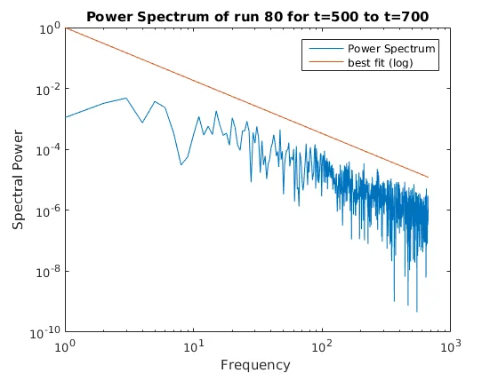
The power spectrum scaling exponent β is calculated by estimating the slope of the power spectrum S(f) plotted on logarithmic axes:
The power spectrum is approximated by the periodogram (the squared magnitude of the Fast Fourier Transform). The exponent is estimated by fitting a line to the periodogram in the frequency range 10-2 ≤ f ≤ 10-1, corresponding to time scales of 10 to 100 units.
function pse_value = PSE(Y)
%% PSE - Estimate β from power spectrum slope
% For S(f) ~ f^(-β): β=0 for white noise, β=2 for Brownian motion

    % Compute periodogram
    [pxx, f] = periodogram(Y, [], [], 1);

    % Remove DC component
    f = f(2:end);
    pxx = pxx(2:end);

    % Fit line in log-log space
    % Frequency range [0.01, 0.1] chosen for AR(1) processes
    window = (f <= 0.1) & (f >= 0.01);

    logf = log10(f(window));
    logp = log10(pxx(window));

    pfit = polyfit(logf, logp, 1);
    pse_value = -pfit(1);  % Negative slope = positive β
end
Validation on Model Data
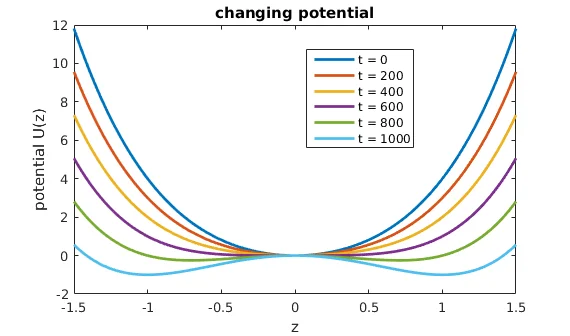
The PS indicator was first validated on a classical pitchfork bifurcation model:
This system has a stable equilibrium at z=0 for t<600, then bifurcates into a double-well potential. All three indicators (ACF1, DFA, PS) successfully detected the approaching bifurcation, with the ACF1 indicator providing the clearest signal.
Application: Tropical Cyclones
The real test came when applying these indicators to sea-level pressure data from 14 major tropical cyclones at landfall. The data was obtained from the HadISD weather station dataset, selecting stations within 2km of landfall locations.
Tropical Cyclones Analysed:
Atlantic hurricanes: Andrew (1992), Opal (1995), Floyd (1999), Charley (2004), Frances (2004), Jeanne (2004), Katrina (2005), Rita (2005), Ivan (2006), Ernesto (2006)
Typhoons: Zeb (1998), Megi (2010), Flo (1990); Cyclone Hudhud (2014)

Key Finding: PS Succeeds Where ACF1 Fails
The striking result was that the ACF1 indicator failed to provide any clear early warning signal for the cyclone data, while the PS indicator showed a clear rising trend starting approximately 50 hours before the minimum pressure.
Why did ACF1 fail? The sea-level pressure data contains strong 12-hour tidal oscillations. These periodic components create a high "background correlation" that masks the critical slowing down signal. The PS indicator, by operating in the frequency domain, is naturally insensitive to these periodic components.
Sensitivity Analysis
An important aspect of the sliding window method is the choice of window size. A sensitivity analysis revealed an interesting pattern: the PS indicator's performance varied periodically with window size, with optimal performance at window sizes of approximately 12n±1 for integer n.
This periodic pattern directly reflects the 12-hour tidal oscillations in the pressure data. Window sizes that are multiples of the oscillation period capture complete cycles and avoid artefacts.
Implementation
function slidingPS = PSE_sliding(data, windowSize)
%% Compute PS exponent in sliding windows across the time series

    n = size(data, 1);
    slidingPS = zeros(n, 1);

    for i = (windowSize + 1):n
        window = data((i - windowSize):i);
        slidingPS(i) = PSE(window);
    end
end

%% Example usage
% Load sea-level pressure data
slp = load('katrina_slp.mat');

% Calculate PS indicator with 100-hour window
ps_indicator = PSE_sliding(slp, 100);

% Statistical significance: Mann-Kendall trend test
[tau, p] = mannkendall(ps_indicator(101:end));
Conclusions
Key Contributions
- Introduced the power spectrum (PS) scaling exponent as a novel EWS indicator
- Demonstrated analytical relationship to established ACF and DFA indicators
- Showed PS indicator detects EWS where ACF1 fails due to periodic oscillations
- First application of EWS methods to tropical cyclone prediction
- Identified optimal window sizes related to data periodicity
This work opened up new possibilities for early warning signal detection in systems with complex periodicities, which are ubiquitous in ecological and geophysical contexts. The PS indicator has since been further developed and applied to multivariate systems and paleoclimate data.
Citation: Prettyman, J., Kuna, T., & Livina, V. (2018). A novel scaling indicator of early warning signals helps anticipate tropical cyclones.EPL (Europhysics Letters), 121(1), 10002.