Power Spectrum Scaling and Critical Slowing Down
Published in Environmental Research Letters, October 2021. Read the paper.
Authors: Joshua Prettyman, Tobia Kuna, Valerie Livina
Summary
This paper provides the rigorous analytical foundation for using the power spectrum (PS) scaling exponent as a tipping point indicator. A key insight is that the PS indicator is useful even when the power spectrum doesn't exhibit true power-law scaling — which is the case for most real dynamical systems.
Most importantly, the paper demonstrates that the PS indicator is remarkably robust against trends and periodic oscillations in the data, making it particularly valuable for ecological and geophysical systems with seasonal or diurnal cycles.
The AR(1) Model of Critical Slowing Down
Critical slowing down (CSD) is commonly modelled using a lag-1 autoregressive (AR(1)) process:
where μ is the autoregressive parameter (related to the return rate), σ is the noise amplitude, and η_n is white noise. As a system approaches a tipping point, μ increases toward 1 — this is the "slowing down" as the system takes longer to return to equilibrium.
Power Spectrum of AR(1)
The power spectrum of an AR(1) process has an analytical form:
This is not a power law. It exhibits a crossover between "white noise" (flat) behaviour at low frequencies and "red noise" (decreasing) behaviour at higher frequencies. Nevertheless, estimating a scaling exponent in this regime proves to be a valid EWS indicator.
Determining the Optimal Frequency Range
A critical question for practical implementation: In what frequency range should we estimate the PS exponent? By differentiating the log-log power spectrum, I derived an expression for the PS indicator as a function of frequency and autoregressive parameter:
The maximum value of B_f(μ) occurs when μ = 1 (at the tipping point) and approaches 2 as f → 0. For the indicator to be useful, we need a frequency range where:
- The indicator shows significant change as μ varies from 0 to 1
- The periodogram is reliable (not too noisy at very low frequencies)
Analysis shows the optimal range is 10⁻² ≤ f ≤ 10⁻¹ (corresponding to time scales of 10 to 100 units). In this range, the PS indicator increases monotonically as CSD progresses.
Validity Without Power-Law Scaling
A key theoretical contribution is proving that estimating a "scaling exponent" is meaningful even when true power-law scaling doesn't exist. I demonstrated this with two cases:
1. Sum of Red and White Noise
For a signal z(t) that is the sum of a random walk W(t) and white noise η(t):
The power spectrum shows a clear crossover, dominated by red noise at low frequencies and white noise at high frequencies. As μ decreases (less white noise), the PS exponent estimated in the crossover region increases — successfully tracking the "reddening" of the signal.
2. AR(1) Process with Changing Parameter
For AR(1) processes with μ ranging from 0 to 1, I derived the exact relationship between μ and the estimated PS exponent β when using the optimal frequency range:
Numerical experiments confirmed that the estimated exponent closely follows this theoretical curve, validating the PS indicator for CSD detection.
Sensitivity Analysis
Sensitivity to Time Series Length
Comparing the PS indicator to the standard ACF1 indicator as estimators of the AR(1) parameter μ reveals an interesting trade-off:
| Series Length | ACF1 Error | PS Error |
|---|---|---|
| 10² | Low | High |
| 10³ | Low | Moderate |
| 10⁵ | Low | Low |
For short time series, ACF1 is more accurate. However, this changes dramatically when the data contains trends or oscillations.
Robustness to Trends
When a parabolic trend is added to AR(1) data, the ACF1 indicator's performance degrades significantly — it consistently overestimates the AR parameter because the trend creates spurious correlation.
The PS indicator, by contrast, shows no degradation for time series longer than 10³ points. The trend affects only very low frequencies, which fall outside the estimation range.
Robustness to Periodic Oscillations
This is the most striking result. When sine waves are superimposed on AR(1) data:
% Original AR(1)
z1(t) = μ·z1(t-1) + η(t)

% AR(1) + simple sine wave
z2(t) = z1(t) + sin(t)

% AR(1) + complex periodic function
z3(t) = z1(t) + 2·sin(50t) + 3·sin(7t)| Indicator | Pure AR(1) | + Simple Sine | + Complex Periodic |
|---|---|---|---|
| ACF1 | Accurate | Biased | Biased |
| DFA | Accurate | Biased | Biased |
| PS | Accurate | Accurate | Accurate |
The PS indicator is practically unchanged when periodic components are added. Oscillations create spikes in the periodogram at specific frequencies, but these are averaged out in the linear fit. This makes the PS indicator ideal for systems with tidal, diurnal, or seasonal cycles.
Application to Paleoclimate Data
The methods were tested on the GISP2 δ¹⁸O ice-core record from Greenland, which contains evidence of the Bølling warming event approximately 14,700 years before present — a dramatic temperature transition at the end of the last ice age.
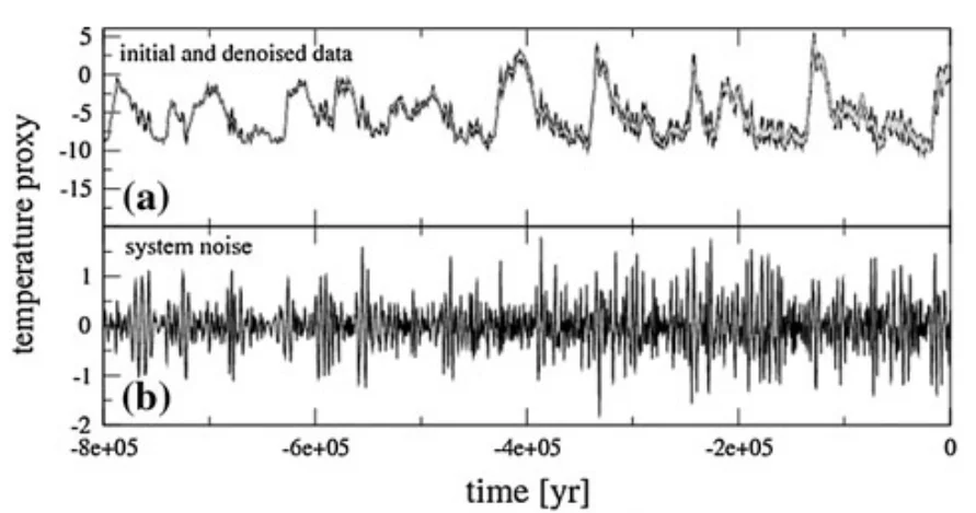
Previous work by Lenton et al. had detected early warning signals in this data using DFA. Applying the PS indicator with a 4,000-year sliding window (approximately 200 data points) confirmed the presence of critical slowing down, though the signal appeared with a lag rather than preceding the transition.
This result highlights a practical limitation: for low-resolution paleoclimate data, the DFA indicator may be more appropriate than the PS indicator, which requires longer time series for optimal performance.
Implications for Modern Climate Monitoring
The PS indicator is most valuable for high-resolution modern data where:
- Time series length exceeds 10³ points
- Tipping points occur over periods of months (with hourly data available)
- Periodic oscillations (tidal, diurnal, seasonal) are difficult to remove
Potential applications include detecting early warning signals for:
- Coral bleaching events linked to ocean temperature increases
- Ecosystem regime shifts in response to climate change
- Extreme weather events monitored by modern meteorological networks
Conclusions
Key Contributions
- Analytical justification for PS indicator based on AR(1) model of CSD
- Determined optimal frequency range (10⁻² to 10⁻¹) for PS estimation
- Proved PS indicator is valid without true power-law scaling
- Demonstrated robustness to trends for series > 10³ points
- Showed remarkable robustness to periodic oscillations
- Validated on paleoclimate ice-core data
- Identified applications for modern high-resolution climate monitoring
This paper completes the theoretical foundation for the PS indicator, establishing when and why it works, and identifying its comparative advantages over traditional methods. The robustness to periodicities makes it particularly valuable for the many ecological and geophysical systems where seasonal and diurnal cycles are present in the data.
Citation: Prettyman, J., Kuna, T., & Livina, V. (2021). Power spectrum scaling as a measure of critical slowing down and precursor to tipping points in dynamical systems.Environmental Research Letters, 16, 114034.